Suppose an educator had a theory which argued that a great deal of learning occurs before children enter grade school or kindergarten. This theory explained that socially disadvantaged children start school intellectually behind other children and are never able to catch up. In order to remedy this situation, he proposes a head-start program, which starts children in a school situation at ages three and four.
A politician reads this theory and feels that it might be true. However, before she is willing to invest the billions of dollars necessary to begin and maintain a head-start program, she demands that the educator demonstrate that the program really does work. At this point the educator calls for the services of a researcher and statistician.
Because this is a fantasy, the following research design would never be used in practice, but it will be used to illustrate the procedure and the logic underlying the hypothesis test. A more appropriate design will be discussed later in the text.
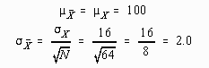
A random sample 64 children is taken from the population of all four-year old children. The children in the sample are all enrolled in the head-start program for a year, at the end of which time they are given a standardized intelligence test. The mean I.Q. of the sample is found to be 103.27.
On the basis of this information, the educator wants to begin a nationwide head-start program. He argues that the average I.Q. in the population is 100 (m=100) and that 103.27 is greater than that. Therefore, the head-start program had an effect of about 103.27-100 or 3.27 I.Q. points. As a result, the billions of dollars necessary for the program would be well invested.
The statistician, being in this case the devil's advocate, is not ready to act so hastily. She wants to know whether chance could have caused the large mean. In other words, the head start program doesn't make a bit of difference. The mean of 103.27 was obtained because the sixty-four students selected for the sample were slightly brighter than average. She argues that this possibility must be ruled out before any action is taken. If it is not possible to completely rule out this possibility, she argues that although possible, the likelihood must be small enough that the risk of making a wrong decision outweighs possible benefits of making a correct decision.
To determine if chance could have caused the difference, the hypothesis test proceeds as a thought experiment. First, the statistician assumes that there were no effects; in this case, that the head-start program didn't work. She then creates a model of what the world would look like if the experiment were performed an infinite number of times under the assumption of no effects. The sampling distribution of the mean is used as this model. The reasoning goes something like this:
Population model assuming no effects
Sampling distribution assuming no effects and N = 64
Results of the study
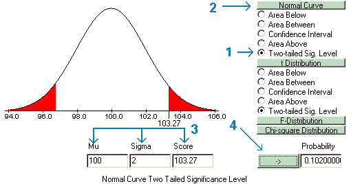
The researcher then compares the results of the actual experiment with those expected from the model, given there were no effects and the experiment was repeated an infinite number of times. The Probability Calculator is used to find the probability of the results of the study given the model of no effect. The probability of finding a result equal to or greater than the actual result is called an exact significance level. It is standard practice to find a two-tailed significance level, taking the total area under the curve both above the score and below a mirror image of the score. In the illustration below, the probability of a score greater than 103.27 or less than 96.73 is .102, or greater than one in ten. The researcher concludes that the model of no effects was not unlikely enough to reject and therefore could explain the results.
Of critical importance is the question "How unlikely do the results have to be before they are unlikely enough?" The researcher must answer this question before the analysis is started and the answer is stated as a probability, called alpha. Alpha is the probability of rejecting the null hypothesis given that the null hypothesis is true, or in other words, the probability of deciding that the effects are real when if fact chance caused the results. An almost universally accepted default value for alpha is .05, although a later chapter deals with the reasons for selections of alternative values for alpha. Unless stated otherwise, the value for alpha will be assumed to be .05.
If the exact significance level is greater than alpha, then the decision of the hypothesis test will always be to retain the null hypothesis. If the exact significance level is less than alpha, then the null hypothesis will be rejected and the alternative hypothesis accepted. In this case, because the value of the exact significance level (.102) is greater than alpha (.05), the null hypothesis must be retained. Therefore, because chance could explain the results, the educator was premature in deciding that head-start had a real effect.
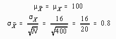
Suppose that the researcher changed the experiment. Instead of a sample of sixty-four children, the sample was increased to N=400 four-year old children. Furthermore, this sample had the same mean (![]() ) at the conclusion as had the previous study. The statistician must now change the model to reflect the larger sample size.
) at the conclusion as had the previous study. The statistician must now change the model to reflect the larger sample size.
Population model assuming no effects
Sampling distribution assuming no effects and N = 400
Results of the study
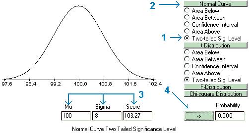
The conclusion reached by the statistician states that it is highly unlikely the model could explain the results. The model of chance is rejected and the reality of effects accepted. Why? The mean that resulted from the study fell far in the tail of the sampling distribution. The following illustration computes the probability of the results given the model of no effects. Although there is area above the value of 103.27 and below the value of 96.73 on this curve, it is too small to register within the display capabilities of the Probability Calculator, thus the probability that results is set to 0, as this figure shows:
The exact significance level, in this case shown as 0.0, is certainly less than alpha, so the null hypothesis must be rejected and the alternative hypothesis accepted. The exact significance level is never exactly equal to zero, as there is always some area under the tails of the curve no matter how far in the tail the score falls. Often the area is so small that it doesn't register in three decimal places and will be shown as .000. In these cases, unless alpha is set to an extremely small value, the null hypothesis will always be rejected.
The different conclusions reached in these two studies may seem contradictory. A little reflection, however, reveals that the second study was based on a much larger sample size (400 versus 64). As such, the researcher is rewarded for doing more careful work and taking a larger sample. The sampling distribution of the mean specifies the nature of the reward.
At this point the question of "how unlikely must the results be in order to reject the model of no effects?" must be answered. In the first example of this chapter the probability of finding a mean of 103.27 given the null hypothesis was true was found to be .102, while in the second it was very close to zero. In the first case the model of no effects was retained, while in the second it was rejected. The question where to draw the line between rejecting and retaining the null hypothesis takes on a critical importance.
Setting the value called "alpha" (a) before the study begins establishes the line between rejecting and retaining the null hypothesis. Alpha is the probability of rejecting the null hypothesis when in fact the null hypothesis is true. Another way of describing alpha is the probability of saying there really were effects when in fact there weren't. In the case of the Head Start Study, alpha would be the probability of finding that Head Start works when if fact it does not.
The decision about whether or not to reject the null hypothesis model is made by comparing the probability (usually designated by "sig.") of the results of the study given the null hypothesis model is true with the value of alpha. The "sig." level has also been termed the exact significance level. If the value of "sig." is less than the value of alpha, the null hypothesis is rejected, otherwise it is retained.
The selection of a value for alpha is arbitrary, but must be done before the study is conducted. It is possible, for example, that the researcher could have set the value of alpha to .25 before the beginning of the Head Start study and thus rejected the null hypothesis in the first example. This would be the case because the value of sig. = .102 is less than the value of alpha = .25. Before the study began, however, the researcher would have to be willing to take the risk that 25 times out of 100 he or she would say they found that Head Start worked when in fact it did not.
While in theory the selection of alpha is arbitrary, in practice it is not. Because journals will generally not accept for publication articles where alpha is set larger than .05 and scientists in general don't want to waste time worrying about results that were due to chance or sampling error, researchers generally use a default value of alpha equal to .05. When in doubt, setting the value of alpha to .05 will generally be the correct decision. A later chapter in this text, however, will discuss in detail why a researcher might want to set the value of alpha to something other than .05.
At this point it should also be pointed out that we are discussing statistical significance: whether or not the results might have occurred by chance. The second question, that of practical significance, occurs only after an affirmative decision about the reality of the effects. The practical significance question is tackled by the politician, who must decide whether the effects are large enough to be worth the money to begin and maintain the program. Even though head-start works, the money may be better spent in programs for health of the aged or for more nuclear submarines. In short, this is a political and practical decision made by people and not statistical procedures.
This chapter illustrated a significance test comparing a single mean to a population parameter (
![]() ).
).
A model of what the world looks like - given that there were no effects and that the experiment was repeated an infinite number of times - was created using the sampling distribution of the mean.
The mean of the experiment was compared to the model to decide whether the effects were due to chance or whether another explanation was necessary (the effects were real). In the first case, the decision was made to retain the model. It could explain the results. In the second case, the decision was to reject the model and accept the reality of the effect.
Finally, a the difference between statistical significance and practical significance was discussed.