A superintendent in a medium size school has a problem. The mathematics scores on nationally standardized achievement tests such as the SAT and ACT of the students attending her school are lower than the national average. The school board members, who don't care whether the football or basketball teams win or not, are greatly concerned about this deficiency. The superintendent fears that if the situation is not corrected, she will lose her job before long.
As the superintendent was sitting in her office wondering what to do, a salesperson approached with a briefcase and a sales pitch. The salesperson had heard about the problem of the mathematics scores and was prepared to offer the superintendent a "deal she couldn't refuse." The deal was teaching machines to teach mathematics, guaranteed to increase the mathematics scores of the students. In addition, the machines never take breaks or demand a pay increase.
The superintendent agreed that the machines might work, but was concerned about the cost. The salesperson finally wrote some figures. Since there were about 1000 students in the school and one machine was needed for every ten students, the school would need about one hundred machines. At a cost of $10,000 per machine, the total cost to the school would be about $1,000,000. As the superintendent picked herself up off the floor, she said she would consider the offer, but didn't think the school board would go for such a big expenditure without prior evidence that the machines actually worked. Besides, how did she know that the company that manufactures the machines might not go bankrupt in the next year, meaning the school would be stuck with a million dollar's worth of useless electronic junk?
The salesperson was prepared, making an offer to lease ten machines for testing purposes to the school for one year at a cost of $500 each. At the end of a year, the superintendent would make a decision about the effectiveness of the machines. If they worked, she would pitch them to the school board; if not, then she would return the machines with no further obligation.
An experimental design was agreed upon. One hundred students would be randomly selected from the student population and would be taught using the machines for one year. At the end of the year, the mean mathematics scores of those students would be compared to the mean scores of the students who did not use the machine. If the means were different enough, the machines would be purchased. (The astute statistics student will recognize this as a nested t-test.)
In order to help decide how different the two means would have to be in order to buy the machines, the superintendent did a theoretical analysis of the decision process. Her analysis is presented in the following decision box.
| "Real World" | ||
|---|---|---|
| DECISION | The machines do NOT work. | The machines work. |
| Buy the machines. Decide the machines work. |
(1.) Type I ERROR probability=a |
(4.) CORRECT probability= 1-b "power" |
| Do not buy the machines. Decide that the machines do not work |
(2.) CORRECT probability=1-a |
(3.) Type II ERROR probability=b |
The decision box has the decision that the superintendent must make in the left column. For simplicity's sake, only two possibilities are permitted: either buy all the machines or buy none of the machines. The other two column titles represent "the state of the real world". The state of the real world can never be truly known, because if it were known whether or not the machines worked, there would be no point in doing the experiment. The four "Real World" cells represent various places one could be, depending upon the state of the world and the decision made. Each cell will be discussed in turn.
1. Buying the machines when they do not work.
This is called a Type I error and in this case is very costly ($1,000,000). The probability of this type of error is a, also called the significance level, and is directly controlled by the experimenter. Before the experiment begins, the experimenter directly sets the value of a. In this example the value of awould be set low, lower than the usual value of .05, perhaps as low as .0001, which means that one time out of 10,000 the experimenter would buy the machines when they didn't work.
2. Not buying the machines when they really didn't work.
This is a correct decision, made with probability 1- awhen in fact the teaching machines don't work and the machines are not purchased.
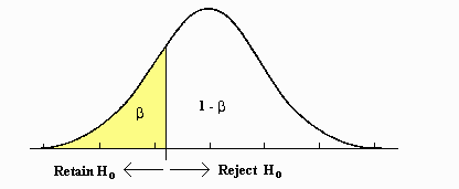
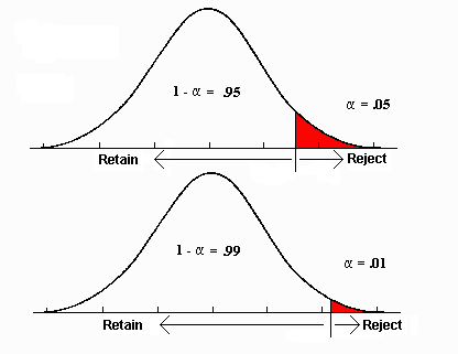
The relationship between the probabilities in these two decision boxes can be illustrated (see the following figures) using the sampling distribution when the null hypothesis is true. The decision point is set by a, the area in the tail or tails of the distribution. Setting a smaller moves the decision point further into the tails of the distribution as you can see in the second distribution.
3. Not buying the machines when they really work.
This is called a Type II error and is made with probability b . The value of b is not directly set by the experimenter, but is a function of a number of factors, including the size of a, the size of the effect, the size of the sample, and the variance of the original distribution. The value of b is inversely related to the value of a: the smaller the value of a, the larger the value of b. It can now be seen that setting the value of ato a small value was not done without cost, as the value of b is increased.
4. Buying the machines when they really work.
This is the cell where the experimenter would usually like to be. The probability of making this correct decision is 1-b and is given the name "power." Because a was set low, b would be high, and as a result 1-b would be low. Thus it would be unlikely that the superintendent would buy the machines, even if they did work.
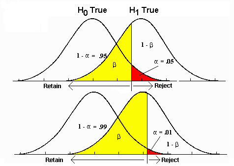
The relationship between the probability of a Type II error (b) and power (1-b) is illustrated in the following sampling distribution when there actually was an effect.
The relationship between the size of aand b can be seen in the following illustration combining the two previous distributions into overlapping distributions, the top graph with a=.05 and the bottom with a=.01.
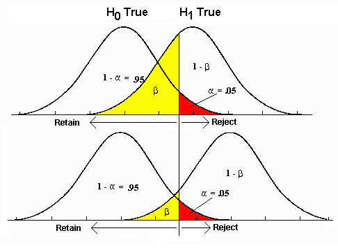
The size of the effect is the difference between the center points (m) of the two distributions. As the size of the effect is increased, the size of beta is decreased.
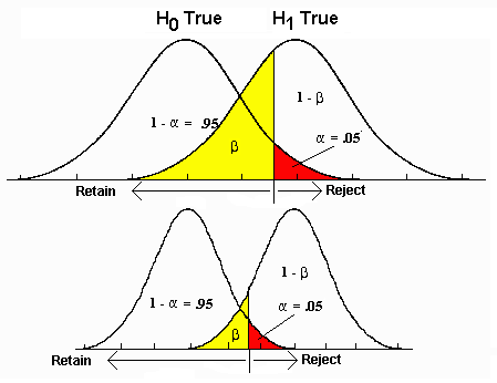
When the error variance of the scores is decreased and everything else remains constant, the probability of a type II error is decreased, as illustrated here:
The interactive exercise designed to allow exploration of the relationships between alpha, size of effects, size of sample (N), size of error, and beta can now be understood. The values of alpha, size of effects, size of sample, and size of error can all be adjusted with the appropriate scroll bars. When one of these values is changed, the graphs will change and the value of beta will be re-computed. The area representing the value of alpha on the graph is drawn in dark gray. The area representing beta is drawn in dark blue, while the corresponding value of power is represented by the light blue area. Use this exercise to verify:
The size of the increase or decrease in beta is a complex function of changes in all of the other values. For example, changes in the size of the sample may have either small or large effects on beta depending upon the other values. If a large treatment effect and small error is present in the experiment, then changes in the sample size are going to have a small effect.
As might be expected, in the previous situation the superintendent chose not to purchase the teaching machines, because she had essentially stacked the deck against deciding that there were any effects. When she described the experiment and the result to the salesperson the next year, the salesperson listened carefully and understood the reason why a had been set so low.
The salesperson had a new offer to make, however. Because of an advance in microchip technology, the entire teaching machine had been placed on a single integrated circuit. As a result the price had dropped to $500 a machine. Now it would cost the superintendent a total of $50,000 to purchase the machines, a sum that is quite reasonable.
The analysis of the probabilities of the two types of errors revealed that the cost of a Type I error, buying the machines when they really don't work ($50,000), is small when compared to the loss encountered in a Type II error, when the machines are not purchased when in fact they do work, although it is difficult to put into dollars the cost of the students not learning to their highest potential.
In any case, the superintendent would probably set the value of ato a fairly large value (.10 perhaps) relative to the standard value of .05. This would have the effect of decreasing the value of b and increasing the power (1-b) of the experiment. Thus the decision to buy the machines would be made more often if in fact the machines worked. The experiment was repeated the next year under the same conditions as the previous year, except that the size of a) was set to .10.
The results of the significance test indicated that the means were significantly different, the null hypothesis was rejected, and a decision about the reality of effects made. The machines were purchased, the salesperson earned a commission, the math scores of the students increased, and everyone lived happily ever after.
The analysis of the reality of the effects of the teaching machines may be generalized to all significance tests. Rather than buying or not buying the machines, you reject or retain the null hypothesis. In the "real world," rather than the machines working or not working, the null hypothesis is true or false. The following decision box presents the choices representing significance tests in general.
| "Real World" | ||
|---|---|---|
| DECISION | NULL TRUE ALTERNATIVE FALSE No Effects |
NULL FALSE ALTERNATIVE TRUE Real Effects |
| Reject Null Accept Alternative Decide there are real effects. |
Type I ERROR probability=a |
CORRECT probability=1-b "power" |
| Retain Null Retain Alternative Decide that no effects were discovered. |
CORRECT probability=1-a |
Type II ERROR probability=b |
When doing an hypothesis test, two types of decision errors are possible. The first, called a Type I error, occurs when the null hypothesis is rejected when in fact it is true. The probability of a Type I error is called alpha and symbolized by a. Alpha is directly set by the researcher with a generally accepted default value of .05. The second type of error is called a Type II error and occurs when the researcher retains the null hypothesis when in fact it is false. The probability of a Type II error is called beta and symbolized by b. The value of beta is indirectly set by the researcher and depends upon four values, including: alpha, effect size, sample size, and error variance. In general, while the size of alpha is known, the size of beta can only be imprecisely estimated.
It is not difficult to conceive of situations where the default value of .05 for alpha should be abandoned for values that take into account the relative costs of each type of error. Since the probabilities of alpha and beta are inversely related, if the cost of a Type I error is high relative to the cost of a Type II error, then the probability of a Type I error (a) should be set relatively low. If the cost of a Type I error is low relative to the cost of a Type II error, then the probability of a Type I error (a) should be set relatively high.