The hypothesis tested when testing a single correlation coefficient is that linear relationship exists between two variables, x and y, as measured by the correlation coefficient (r). The null hypothesis states that no linear relationship exists between the two variables. As in all hypothesis tests, the goal is to reject the null hypothesis and accept the alternative hypothesis; in other words, to decide that an effect, in this case a relationship, exists
Suppose a study was performed which examined the relationship between life-satisfaction and attitude toward boxing. The attitude toward boxing measured by the following statement on a questionnaire:
1. I enjoy watching a good boxing match.
Life-satisfaction is measured with the following statement:
2. I am pretty much satisfied with my life.
Both items were measured with the following scale:
1=Strongly Disagree 2=Disagree 3=No Opinion 4=Agree 5=Strongly Agree
The questionnaire was given to N=33 people. The obtained correlation coefficient between these two variables was r=-.30. Because the correlation is negative we conclude that the people who said they enjoyed watching a boxing match were less satisfied with their lives. The corollary, that individuals who said they were satisfied with their lives did not say they enjoyed watching boxing, is also true. On the basis of this evidence the researcher argues that there was a relationship between the two variables.
Before she could decide that there was a relationship, however, a hypothesis test had to be performed to negate, or at least make improbable, the hypothesis that the results were due to chance. The ever-present devil's advocate argues that there really is no relationship between the two variables; the obtained correlation was due to chance. The researcher just happened to select 33 people who had a negative correlation between these two variables. If another sample were taken, the correlation was just as likely to be positive and just as large. Furthermore, if a sample of infinite size (population) was taken and the correlation coefficient computed, the true correlation coefficient would be 0.0. In order to answer this argument, a hypothesis test is needed.
The model of no effects is described by the sampling distribution of a correlation coefficient. In a thought experiment, the study is repeated an infinite number of times using the same two questions and a different sample of 33 individuals each time, assuming the null hypothesis is true. Computing the correlation coefficient each time results in a sampling distribution of the correlation coefficient. This distribution of correlation coefficients can be graphed in a theoretical relative frequency distribution that is similar to the following:
Note that this distribution looks like a normal distribution. It could not be normal, however, because the scores are limited to the range of -1.0 and 1.0.
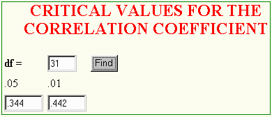
Because the sampling distribution of the correlation coefficient has a unique shape, a computer program, which is included in this book, is used to find values that cut off a given proportion of area. To use the program, you must first find the degrees of freedom using the following formula:
df = N - 2
Enter the the degrees of freedom in the df= box, as shown in the following figure, and, click the Find button
These are the same values that appear in the sampling distribution of the correlation coefficient just presented. The values appearing in the row corresponding to the degrees of freedom are areas (probabilities) falling below the tail(s) of the distribution. In the previous example, .95 area falls between correlations of -.344 and .344, and .99 area between -.422 and .442.
The obtained correlation coefficient is now compared with what would be expected given the model created under the null hypothesis. In the earlier example, the value of -.30 falls inside the critical values of -.344 and .344 that were found using the computer program. Because the obtained correlation coefficient did not fall in the tails of the distribution under the null hypothesis, the model and the corresponding null hypothesis must be retained. The model of no effects could explain the results. The correlation coefficient is not significant at the .05 level.
If the obtained correlation coefficient had been -.55, however, the decision would have been different. In that case the obtained correlation is unlikely given the model, because it falls in the tails of the sampling distribution. The model and corresponding null hypothesis are rejected as unlikely and the alternative hypothesis, that of a real effect, accepted. The obtained correlation is said to be significant at the .05 level.
Hypothesis testing using a correlation coefficient to measure the size of the effect tests whether two variables are linearly related to one another. By finding the likelihood of the obtained correlation coefficient given a model of correlation coefficients when there are no effects, a decision can be made about whether the two variables are linearly related.