Most multivariate statistical methods are built on the foundation of linear transformations. A linear transformation is a weighted combination of scores where each scores is first multiplied by a constant and then the products are summed. In its most general form, a linear transformation appears as follows:
Xi' = w0 + w1X1i + w2X2i + ... + wkXki
where K is the number of different scores for each subject and X' is the linear combination of all the scores for a given individual.
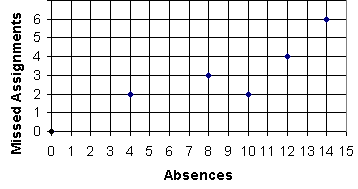
A linear transformation combines a number of scores into a single score. A linear transformation is useful in that it is cognitively simpler to deal with a single number, the transformed score, than it is to deal with many numbers individually. For example, suppose a statistics teacher had records of absences (X1) and number of missed homework assignments (X2) during a semester for six students (N=6).
| Absences | Missed Assignments | |
|---|---|---|
| Student (i) | X1i | X2i |
| 1 | 10 | 2 |
| 2 | 12 | 4 |
| 3 | 8 | 3 |
| 4 | 14 | 6 |
| 5 | 0 | 0 |
| 6 | 4 | 2 |
The teacher wishes to combine these separate measures into a single measure of student tardiness. The teacher could just add the two numbers together, with implied weights of one for each variable. This solution is rejected, however, as more weight would be given to absences than missed assignments because absences have greater variability. The solution, the teacher decides, is to take the sum of one-half of the absences and twice the missed homework assignments. This would result in a linear transformation of the following form:
Xi' = w0 + w1X1i + w2X2i
where: w0 = 0, w1 = .5, and w2 = 2 giving
Xi' = .5X1i + 2X2i
Application of this transformation to the first subject's scores would result in the following:
Xi' = .5X1i + 2X2i
Xi' = .5*10 + 2*2 = 5 + 4 = 9
The following table results when the linear transformation is applied to all scores for each of the six students:
| Absences | Missed Assignments | Tardiness | |
|---|---|---|---|
| Student (i) | X1i | X2i | X'i |
| 1 | 10 | 2 | 9 |
| 2 | 12 | 4 | 14 |
| 3 | 8 | 3 | 10 |
| 4 | 14 | 6 | 19 |
| 5 | 0 | 0 | 0 |
| 6 | 4 | 2 | 6 |
| Mean | 8 | 2.833 | 9.667 |
| s.d. | 5.215 | 2.041 | 6.532 |
| Var. | 27.196 | 4.166 | 42.665 |
As can be seen, student number 4 has the largest measure of tardiness with a score of 19.
As in the section on simple linear transformations, the mean and standard deviation of the transformed scores are related to the mean and standard deviation of the scores combined to create the transformed score. In addition, when transforming more than a single score into a combined score, the correlation coefficient between the scores affects the size of the resulting transformed variance and standard deviation. The formulas that describe the relationship between the means, standard deviations, and variances of the scores are presented below:
![]() ' = w0 + w1
' = w0 + w1 ![]() 1 + w2
1 + w2 ![]() 2
2
sx'2 = w12 s12 + w22 s22 + 2w1w2s1s2r12
Application of these formulas to the example data results in the following, where the correlation (r12)between the X1i and X2i is .902:
![]() ' = w0 + w1
' = w0 + w1 ![]() 1 + w2
1 + w2 ![]() 2
2
![]() ' = 0 + .5*8 + 2*2.833 = 4 + 5.66 = 9.66
' = 0 + .5*8 + 2*2.833 = 4 + 5.66 = 9.66
sx'2 = w12 s12 + w22 s22 + 2*w1w2s1s2r12
sx'2 = .52*5.2152 + 22*2.0412 + 2*.5*2*5.215*2.041*.902
= .25*27.196 + 4*4.166 + 19.202 = 42.665
Note that the values computed with these formulas agree with the actual values presented in an earlier table.
When combining two variables in a linear transformation the variance of the transformed scores is a function of the variances of the individual variables and the correlation between the variables. A number of possibilities exist, depending upon sign of the correlation coefficient and the signs of the weights.
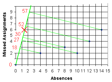
The pairs of data may be represented as points on a scatter plot. For example, the six pairs of example data appear as six points on the following scatter plot.
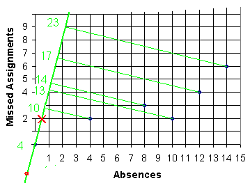
The linear transformation, defined by the equation Xi' = w0 + w1X1i + w2X2i, may be represented as a rotation of the axes of the scatter plot. The first step is to identify the point (w1,w2) on the graph. In the example transformation, Xi' = .5*X1i + 2*X2i, this point would be (.5,2). On the example below this point is drawn using a red X.
The next step is to draw a line from the origin (0,0) through the point just identified. This line will be the rotated axis and on the example below, it is the green line that appears at an angle to the original y-axis.
The final step is to project the points on the scatter plot onto the new axis by drawing a line perpendicular from the new axis through the points. The point where these lines cross the new axis will be their transformed value. For example, the point (8,3) is transformed into a value of 10 (.5*8 + 2*3 = 10) on the new axis. Note that the relative spacing between the projected points on the graph below preserves the differences between the transformed values, i.e. the distance between 6 and 10 is the same as the distance between 10 and 14.
Adding a constant term (w0) other than zero moves the origin on the new axis. Performing a linear transformation of the following form:
Xi' = w0 + w1X1i + w2X2i
where: w0 = 4, w1 = .5, and w2 = 2 giving
Xi' = 4 + .5X1i + 2X2i
Application of this transformation to the first subject's scores would result in the following:
Xi' = 4 + .5X1i + 2X2i
Xi' = 4 + .5*10 + 2*2 = 5 + 4 = 13
The following table results when the linear transformation is applied to all scores for each of the six students:
| Absences | Missed Assignments | Tardiness | |
|---|---|---|---|
| Student (i) | X1i | X2i | X'i |
| 1 | 10 | 2 | 13 |
| 2 | 12 | 4 | 17 |
| 3 | 8 | 3 | 14 |
| 4 | 14 | 6 | 23 |
| 5 | 0 | 0 | 4 |
| 6 | 4 | 2 | 10 |
| Mean | 8 | 2.833 | 13.667 |
| s.d. | 5.215 | 2.041 | 6.532 |
| Var. | 27.196 | 4.166 | 42.665 |
This transformation can be visualized on the following scatter plot. Note that the rotated axis is identical to the previous illustration, but the origin, shown as a red dot, has been moved.
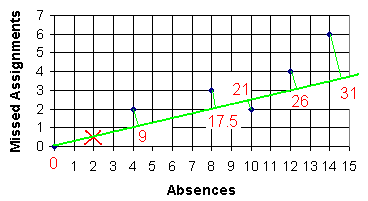
Another linear transformation of the following form will now be illustrated:
Xi' = w0 + w1X1i + w2X2i
where: w0 = 0, w1 = 2, and w2 = .5 giving
Xi' = 2X1i + .5X2i
Application of this transformation to the first subject's scores would result in the following:
Xi' = 2X1i + .5X2i
Xi' = 2*10 + .5*2 = 20 + 1 = 21
The following table results when the linear transformation is applied to all scores for each of the six students:
| Absences | Missed Assignments | Tardiness | |
|---|---|---|---|
| Student (i) | X1i | X2i | X'i |
| 1 | 10 | 2 | 21 |
| 2 | 12 | 4 | 26 |
| 3 | 8 | 3 | 17.5 |
| 4 | 14 | 6 | 31 |
| 5 | 0 | 0 | 0 |
| 6 | 4 | 2 | 9 |
| Mean | 8 | 2.833 | 17.42 |
| s.d. | 5.215 | 2.041 | 11.36 |
| Var. | 27.196 | 4.166 | 129.04 |
As before, the rotated axis is drawn by first identifying a point corresponding to the weights of the transformation (2, .5) and then drawing a line perpendicular to the new axis through the points. Note that the ordering of the points on the transformation axis is slightly different from the ordering in the previous examples. Note also that the rotated axis defining the transformation seems to "pass through" the points to a much greater extent than the first transformations. Note also that the variance of the resulting points has increased.
Another transformation may be selected that takes the form:
Xi' = 1.5 X1i + 6 X2i.
The transformed values are presented in the table below. Note that the new values of both w1 and w2 are three times the values of the first transformation illustrated in this chapter. The transformed scores and resulting mean and standard deviation are all three times the size of the first transformation.
| Student (i) | X1i | X2i | X'i |
| 1 | 10 | 2 | 27 |
| 2 | 12 | 4 | 52 |
| 3 | 8 | 3 | 30 |
| 4 | 14 | 6 | 57 |
| 5 | 0 | 0 | 0 |
| 6 | 4 | 2 | 18 |
| Mean | 8 | 2.833 | 29 |
| s. d. | 5.215 | 2.041 | 19.596 |
The line defining the transformation is drawn on the scatter plot below. Note that the rotated axis defining the transformation is identical to the first transformation discussed in this chapter.
In some ways, then, all transformations where the weights are a multiple of another transformation are similar, sharing the same rotated axis. The correlation coefficient between the resulting values of such transformations will be 1.0. In general, if w1/w2 = w1*/w2*, then the transformations are similar except for a multiplicative constant.
Statisticians are interested in the linear transformation that maximizes the obtained variance. It is obvious, however, that increasing the size of the transformation weights will arbitrarily increase the variance of the obtained transformed scores. In order to control for this artifact, the scores will first be mean centered and then restrictions will be placed on the transformation weights so that similar transformations sharing the same rotation of the axis will be treated as a single transformation.
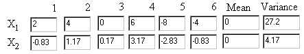
A linear transformation is called a mean centered transformation if the mean is subtracted from the scores before the linear transformation is done. Mean centering basically allows a cleaner view of the data. The following table presents the results of mean centering the example data and applying the transformation Xi' = .5X1i + 2X2i.
| Score | X1 | X1 - |
X2 | X2 - |
X' |
| 1 | 10 | 2 | 2 | -.833 | -.667 |
| 2 | 12 | 4 | 4 | 1.167 | 4.333 |
| 3 | 8 | 0 | 3 | .167 | .333 |
| 4 | 14 | 6 | 6 | 3.167 | 9.333 |
| 5 | 0 | -8 | 0 | -2.833 | -9.667 |
| 6 | 4 | -4 | 2 | -.833 | -3.667 |
| Mean | 8 | 0 | 2.833 | 0 | 0 |
| s.d. | 5.215 | 5.125 | 2.041 | 2.041 | 6.531 |
| Variance | 27.2 | 27.2 | 4.167 | 4.167 | 42.650 |
Note that the mean of the transformation is zero, but the standard deviation and variance are identical to those previously calculated using the same transformation weights. Mean centering the data has the effect of changing the origin of the scatter plot to the intersection of the two means.
As stated earlier, one possible goal of performing a linear transformation is to maximize the variance of the transformed scores. It was observed, however, that simply making the transformation weights larger could arbitrarily increase the variance of the transformed variable and that some sort of restriction limiting the size of the weights would need to be imposed. Normalizing the transformation weights imposes that restriction.
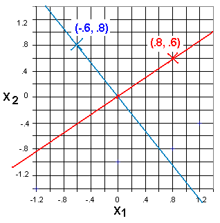
A linear transformation is said to be normalized if the sum of the squared transformation weights is equal to one, not including w0. In the case of two variables, any transformation where w12 + w22 = 1 would be a normalized linear transformation. For example, the linear transformation X'i = .8X1i + .6X2i would be a normalized linear transformation because w12 + w22 = .82 + .62 = .64 + .36 = 1.
Any linear transformation may be normalized by applying the following formula to its weights.
For example, the transformation X' = .5X1 + 2X2 could be normalized by transforming the weights to values of
Note that w1'2 + w2'2 = .24252 + .97012 = .0588 + .9411 = .9999 and -w1/w2 = -.5/2 =-.25 = -w1'/w2' = -.2425/.9701 = -.25. The first result implying that the transformation is a normalized linear transformation and the second implying that the same line defines both transformations.
The advantages of mean centering and normalizing a linear transformation include:
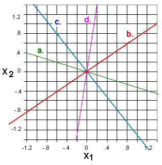
Given that a normalized linear transformation, Xi' = w1X1i + w2X2i, has been defined, there exists a second normalized linear transformation, Xi'' = w1'X1i + w2'X2i, such that w1' = -w2 and w2' = w1. A line that is perpendicular to the line defined by the first normalized transformation will define this second normalized transformation.
The proof that these lines are perpendicular is a fairly simple exercise in geometry, but we will let the illustration below suffice. The red line shows the rotation associated with the first transformation, X' = w1X1 + w2X2 = .8X1 + .6X2, while the blue line shows the second, X'' = w'1X1 + w'2X2 = -.6X1 + .8X2.
In addition, the sum of the transformed variances will be equal to the sum of the variances of the untransformed scores.
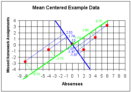
For example, application of the normalized transformation X' = w1X1 + w2X2 = .8X1 + .6X2 and X'' = w'1X1 + w'2X2 = -.6X1 + .8X2 to the mean centered example data results in the following table.
| Score | X1 - |
X2 - |
X' | X'' |
| 1 | 2 | -.833 | 1.10 | -1.866 |
| 2 | 4 | 1.167 | 3.90 | -1.466 |
| 3 | 0 | .167 | .10 | .134 |
| 4 | 6 | 3.167 | 6.70 | -1.066 |
| 5 | -8 | -2.833 | -8.10 | 2.534 |
| 6 | -4 | -.833 | -3.70 | 1.737 |
| Mean | 0 | 0 | 0 | 0 |
| s.d. | 5.125 | 2.041 | 5.303 | 1.801 |
| Variance | 27.2 | 4.167 | 28.124 | 3.245 |
Note that both transformations are normalized as w12 + w22 = .82 + .62 = .64 + .36 = 1.00 and w'12 + w'22 = .62 + (-.8)2 = .36 + .64 = 1.00. Note also that the sum of the variances of the untransformed variables (s12 + s22 = 27.2 + 4.167 = 31.367) is equal to the sum of the variances of the transformed variables (s'2 + s''2 = 28.124 + 3.245 = 31.369), at least within rounding error.
The sum of the transformed variances must always equal the sum of the untransformed variances as the following proves.
Where X' = w1X1 + w2X2, X'' = -w'2X1 + w'1X2, and w12 + w22 = 1.00
s'2 + s''2
(w12 s12 + w22 s22 + 2w1w2s1s2r12) + ((-w2)2s12 + w12 s22 + 2(-w2)w1s1s2r12)
w12 s12 + w22 s22 + 2w1w2s1s2r12 + w22s12 + w12 s22 - 2w2w1s1s2r12
w12 s12 + w22 s22 + w22s12 + w12 s22
w12 s12 + w22s12 + w22 s22+ w12 s22
(w12 + w22) s12 + (w22 + w12) s22
s12 + s22
As always, if you are unable (or unwilling) to follow the proofs, you must "believe."
The two transformations presented above may be visualized in a manner similar to that described earlier. Conceptually, the axes are rotated and the points are projected onto the new axes.
It appears the variance of X' might be increased if the axes were rotated clockwise even further than the present transformation. At some point the variance would begin to grow smaller again. Obtaining transformation weights that optimize variance is the problem that the next section addresses.
It was shown earlier that the total variability is unchanged when normalized transformations are done on mean centered data. It was also demonstrated that the distribution of variability changed, that is, X' had greater variance than X''. Mathematically, the question can be asked, "can a transformation be found such that one variable has a maximal amount of variance and the other has a minimal amount of variance?" Optimizing linear transformations such that transformed variables contain a maximal amount of variability is the fundamental problem addressed by eigenvalues and eigenvectors.
Eigenvalues are the variances of the transformations when an optimal (maximal variance) linear transformation has been found. Eigenvectors are the transformation weights of optimal linear transformations.
Mathematical procedures are available to compute eigenvalues and eigenvectors and will be presented shortly. Before these methods are presented, however, a manual method using an interactive computer exercise will be discussed.
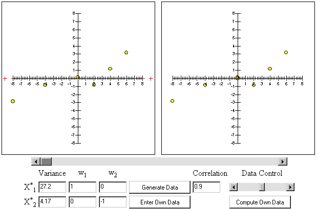
The display of the transformation program has been modified by reducing the data pairs to six and rescaling the axes. After clicking on the "Enter Own Data" button, the first step is to enter the mean centered data. After entering the data, click on the "Compute Own Data" button. The means and variances of the data will appear in the appropriately labeled boxes.
In addition, the following scatter plots, controls, and text boxes will appear. Note that the variances of the transformed variables (X*1 and X*2) are the same as the original variables (X1 and X2) at the start of the program. The weights are set at values w1=1 and w2=0 so that the transformed axes are identical to the original axes.
The program is designed to always generate two sets of perpendicular standardized normal transformations. The user can change the weights in two different ways. Clicking on the large area of the scroll bar causes a fairly large change in the transformation weights.
Clicking on the triangles on either end causes a small change in the transformation weights.
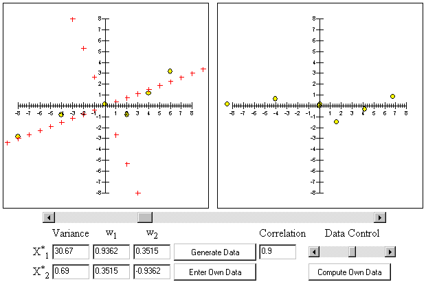
In either case, new weights are selected and the variances of the transformed scores are recomputed and displayed. The points on the scatter plot on the left remain unchanged, but the axes are rotated to display the lines defined by the transformations. The scatter plot on the right displays the plot of the transformed scores.
The goal is to adjust the axes so that the variance of one of the transformed variables is maximized and the other is minimized. This can be accomplished by first changing the weights with fairly large steps. The variance will continue increasing until a certain point has been reached. At this point begin using smaller steps. Continue until the variance begins to decrease. Because of what I believe is rounding error, the program sometimes behaves badly at this level. Be sure to continue in both directions for a number of small steps before deciding that a maximum and minimum variance has been found.
Note that the program automatically normalizes the transformation weights and the sum of the variances remains a constant, no matter what weights are used.
In the example data, the adjustments to the weights were continued until the values in the display were found. Note that the axes pass through the points in the direction that most students intuitively believe is the position of the regression line (it isn't). In this case the eigenvalues would be 30.67 and .69. The two pairs of eigenvectors would be (.936, .352) and (.352, -.936).
Performing a two linear transformations of the following form:
Xi' = w1X1i + w2X2i
where: w1 = .936, and w2 = .352 giving
Xi' .936X1i + .352X2i
and
where: w1 = .352 and w2 = -.936 giving
Xi" = .352X1i - .936X2i
The transformations applied to the example data is shown below. Note that the variances of the two variables are equal to the eigenvalues.
| Score | X1 - |
X2 - |
X' | X'' |
| 1 | 2 | -.833 | 1.579 | 1.48 |
| 2 | 4 | 1.167 | 4.155 | .316 |
| 3 | 0 | .167 | .059 | -.156 |
| 4 | 6 | 3.167 | 6.731 | -.864 |
| 5 | -8 | -2.833 | -8.485 | -.164 |
| 6 | -4 | -.833 | -4.037 | -.628 |
| Mean | 0 | 0 | 0 | 0 |
| s.d. | 5.125 | 2.041 | 5.538 | .835 |
| Variance | 27.2 | 4.167 | 30.672 | .696 |
It should come as no surprise to the student that mathematical procedures have been developed to find exact eigenvalues and eigenvectors of both this relatively simple case of two variables and far more complicated situations involving linear combinations of many variables. The procedures involve matrix algebra and are beyond the scope of this text. The interested reader will find a much more complete and mathematical treatment in Johnson and Wickren, 1996.
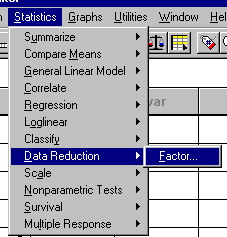
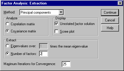
Eigenvalues and eigenvectors can be found using the Factor Analysis package of SPSS. Starting with the raw data as variables in a data matrix, the next step is to click on Analyze/Data Reduction/Factor. The display should appear as follows:
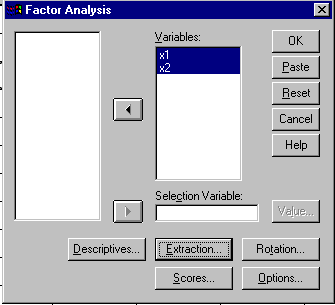
The program will then display the choices associated with the Factor Analysis package. Select the variables that are to be included in the analysis and click them to the right-hand box. At this point some of the default values associated with the "Extraction" button will need to be modified, so clicking on this button gives the following choices:
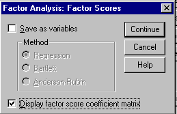
Checking the "Covariance matrix" will result in the analysis of raw data rather than standardized scores. In addition, the computer will be told that 2 factors will be extracted, rather than allowing the computer to automatically decide how many factors will be extracted. Be sure that the "Principal components" is the selected method for factor extraction. Click on "Continue" and the main factor analysis selections should reappear. Click the "Scores" button to modify the output to print tables that will allow the computation of the eigenvectors.
Click on the "Display factor score coefficient matrix" option and then click on "Continue." Back in the main factor analysis display, click on the "OK" button to run the program.
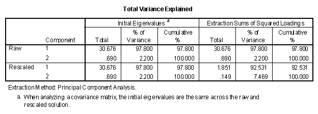
The eigenvalues appear in an output table labeled "Total Variance Explained." Note that the values of 30.676 and .690 closely correspond to what was found by manually rotating the axes.
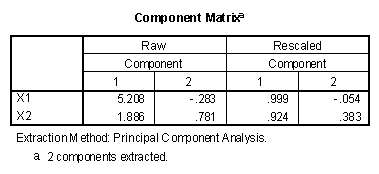
The eigenvectors do not appear directly on the a table in the SPSS output. They may be computed by normalizing the "Raw Components" in the following "Component Matrix" table.
While not exact, these values are within rounding error of the values found using the manual approximation procedure. The student may verify that the "Raw Components" for "2" correspond to the second normalized eigenvector.
Linear transformations are used to simplify the data. In general, if the same amount of information (in this case variance) can be explained by fewer variables, the interpretation will generally be simpler.
Linear transformations are the cornerstone of multivariate statistics. In multiple regression linear transformations are used to find weights that allow many independent variables to predict a single dependent variable. In canonical correlation, both the dependent and independent variables have two or more variables and the goal of the analysis is to find a linear combination of the independent variables which best predicts a linear combination of the dependent variables.
Factor analysis is similarly a linear transformation of many variables. The goal in factor analysis is a description of the variables, rather than prediction of a variable or set of variables. In factor analysis, a combination of weights is selected (extracted), usually with some goal, such as maximizing the variance of the transformed score or maximizing the correlation of the transformed score with all the scores that produce it. In factor analysis, a second combination of weights is then selected which meets the goal of the analysis. This process could continue until the number of transformed variables equals the number of original variable, but usually does not because after a few meaningful transformations, the rest do not make much sense and are discarded. The goal of factor analysis is to explain a set of variables with a few transformed variables
Linear transformation form the cornerstone for many multivariate statistical techniques. Linear transformations of two variables were examined in this chapter. Formulas were presented to compute the mean, standard deviation, and variance of a linear transformation given the weights, means, variances, and correlation coefficient of the original data. Linear transformations were presented graphically as projection of points on a rotated axis.
Mean centering was presented as a way to simplify the data presentation. Standard normalized linear transformations were shown as a means to standardize the weights of a linear transformation with two or more variables. A way to construct a second transformation that was perpendicular to a given standard normalized was shown. It was proven that the sum of the variances of the two perpendicular standard normalized transformation was equal to the sum of the variances of the original variables.
A computer program to manually rotate the axes to find a standard normalized linear transformation that maximized the variance of one of the transformed variables was shown. The resulting variances were called eigenvalues and the weights eigenvectors. A way to find eigenvectors and eigenvalues using SPSS was demonstrated.
Finally, an application of linear transformation was demonstrated using a principal components analysis.